This page will introduce the dynamic analysis function (frequency response analysis and transient response analysis) of Jupiter-Post.

 

1. Introdution of the dynamic analysis function of Jupiter-Post

• You can perform frequency response analysis and transient response analysis on the solver’s real eigenvalue analysis results.
• It is possible to obtain a large number of response results at a very high speed by calculating the response by the modal method.
• It supports ABAQUS, ADVC, Nastran, and SunShine-Solver result output formats.

 

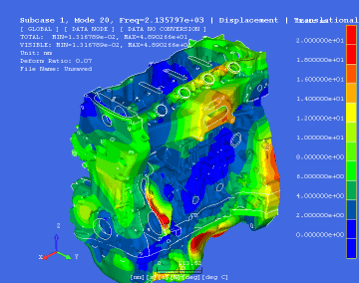
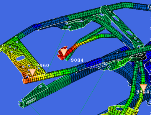
Example of real eigenvalue analysis result

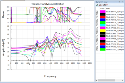
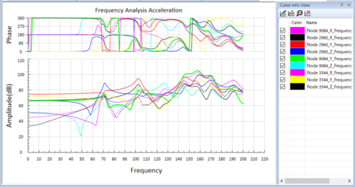
Example of frequency response function result (Jupiter)

 

2. Frequency response analysis function

• It is a frequency response calculation by the modal method.
• You can select multiple vibration points and response points from the GUI.
• The calculation is very fast, and even a large number of response points can be calculated in seconds.
• The exciting force setting conforms to the Nastran RLOAD2 format. You can also input and output in the Nastran bdf file format.
• Check the result by outputting the response result to an XY graph or CSV external file.

 

2.1 Setting vibration conditions

• You can easily specify the vibration point from the GUI.
• The exciting force conforms to the Nastran RLOAD2 format.
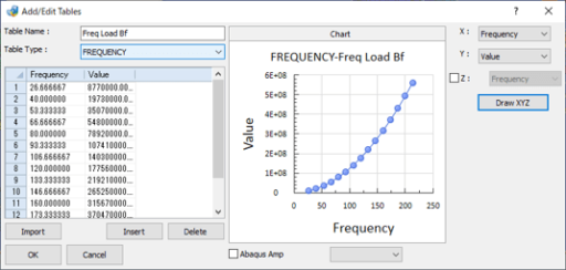
• It also supports the input of frequency tables of Amplitude and Phase.
• It also supports local coordinate system references.
• Unit vibration and centrifugal force can also be set.

Frequency table

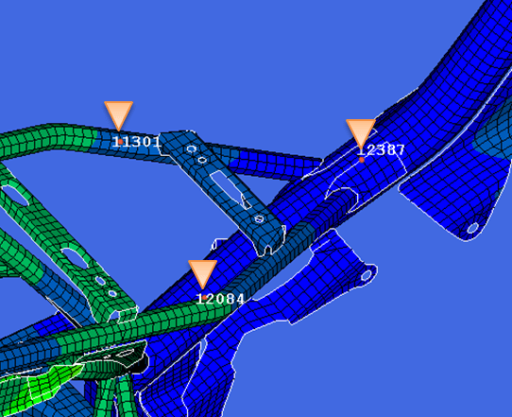
Specifying the vibration points

 

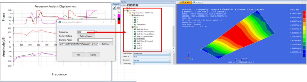
2.2 Response conditions and calculation settings

• You can easily specify the response points from the GUI.
• Execute the calculation by specifying the attenuation coefficient (changeable by the frequency table) and the calculation frequency.
• Results can be specified from displacement, velocity, acceleration and stress.
• It also supports the output as a result of referencing the local coordinate system.

 

Specifying the response point

2.3 Response function output

• The calculation result is displayed as an XY graph. Based on the Bode diagram that displays Amplitude and Phase at the same time, you can change it according to your needs.
• You can output a file in CSV format from the Chart ribbon, and there are various functions such as changing the graph format, displaying / hiding numerical values, and displaying / hiding each result curve.

 

XY graph

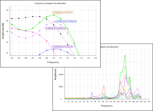
Various functions of the graph

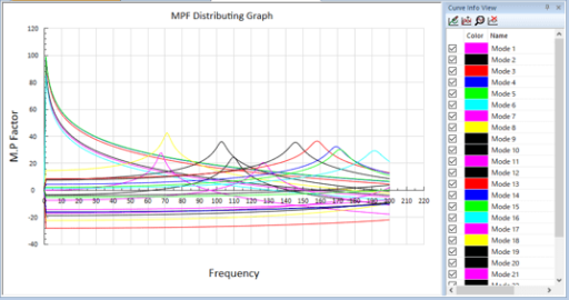
2.4 Displaying MPF functions

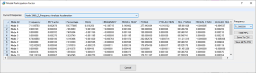
• The MPF (※) of the calculated response curve can be displayed.

　※ MPF（Modal Participation Factor ）

• Select an arbitrary position on the response curve, and the contribution rate for each mode of the specified frequency is displayed in a list. You can also display the contribution curve in the calculated frequency range.

Contribution rate list

Contribution rate curve

2.5 Interactive operation

• Interactive operation can be realized with the command for vibration point response calculation.
• The below demo video showing that the vibration condition and the response condition are set at the same time.

 

 

2.6 SunShine-Frequency response calculation for Solver results

• In the frequency response calculation for the actual eigenvalue analysis result of SunShine-Solver, the following is possible.

　■ Forced vibration

　　Displacement, velocity, and acceleration can be specified for the physical quantity used for vibration in addition to force.

　■ Create the mode animation

　　You can create a result that considers the phase from the results of all the nodes of the specified frequency.

　

 

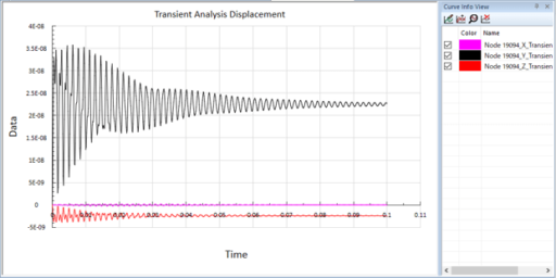
3. Transient response analysis function

• Transient response calculation by modal method.
• You can select multiple vibration points and response points from the GUI.
• The calculation is very fast, and even a large number of response points can be calculated in seconds.
• The exciting force setting conforms to the Nastran TLOAD1 format and TLOAD2 format.
• You can check the result by outputting the response result to an XY graph or CSV external file.

Transient response function result (Jupiter)

 

3.1 Setting of vibration conditions

• You can easily specify the vibration point from the GUI.
• The exciting force conforms to the Nastran TLOAD1 format and the TLOAD2 format.
• It also supports Time table input.
• It also supports local coordinate system references.

 

3.2 Response conditions and calculation settings

• You can easily specify the response point from the GUI.
• Execute the calculation by specifying the attenuation coefficient (changeable depending on the mode) and the calculation time range.
• Results can be specified from displacement, velocity and acceleration.
• It also supports output as a result of referencing the local coordinate system.

 

3.3 Response function output

• The calculation result is displayed as an XY graph.
• The contents of the graph can be output as a file in CSV format.
• There are various functions such as changing the graph format, displaying / hiding numerical values, and displaying / hiding each result curve.